In this post I will describe how I built a neural network to decode morse code. After a day of training it successfully decoded real signals. First I’ll describe the generation of morse code signals, the neural net, and finally the results.
Morse code generation
You want the training data to match the real world as closely as possible. Unfortunately I couldn’t find a dataset with real world labeled morse code. Therefore I wrote a simple morse code generator that simulates a wide variety of signals:
MORSE_CODE_DICT = {'A': '.-', 'B': '-...', ... }

def generate_sample(text_len=10, pitch=500, wpm=20, noise_power=1, amplitude=100, s=None):
  # Reference word is PARIS, 50 dots long
  dot = (60 / wpm) / 50 * SAMPLE_FREQ

  # Add some noise on the length of dash and dot
  def get_dot():
    scale = np.clip(np.random.normal(1, 0.2), 0.5, 2.0)
    return int(dot * scale)

  # The length of a dash is three times the length of a dot.
  def get_dash():
    scale = np.clip(np.random.normal(1, 0.2), 0.5, 2.0)
    return int(3 * dot * scale)

  out = []
  for c in s:
    for m in MORSE_CODE_DICT[c]:
      if m == '.':
        out.append(np.ones(get_dot()))
        out.append(np.zeros(get_dot()))
      elif m == '-':
        out.append(np.ones(get_dash()))
        out.append(np.zeros(get_dot()))
    out.append(np.zeros(2 * get_dot()))
  out = np.hstack(out)

  # Modulation
  t = np.arange(len(out)) / SAMPLE_FREQ
  sine = np.sin(2 * np.pi * t * pitch)
  out = sine * out

  # Add noise
  noise_power = 1e-6 * noise_power * SAMPLE_FREQ / 2
  noise = np.random.normal(scale=np.sqrt(noise_power),
                           size=len(out))
  out = 0.5 * out + noise

  out *= amplitude / 100
  out = np.clip(out, -1, 1)
As can be seen in the code the length of dots and dashes are varied randomly during the sequence to mimic the variations as a human would manually key the morse code. The sequence of dots and dashes is then modulated with a sine wave of variable frequency. Then white noise is added, the amplitude is varied and the output is clipped. During training the parameters to this function are varied randomly.
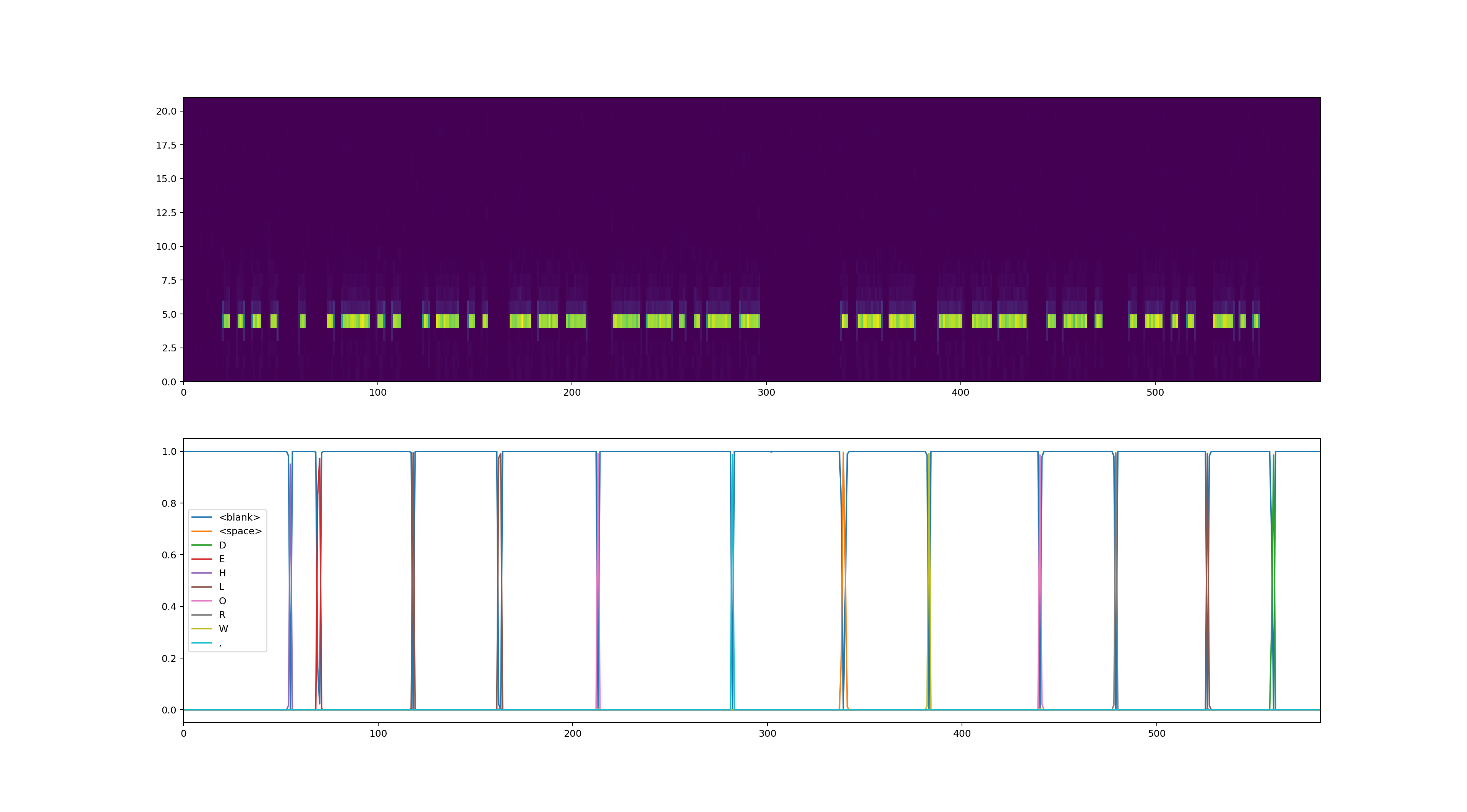
This is an example from the generator for the text “HELLO, WORLD”
Pre-processing
Instead of feeding the audio straight into the neural network some pre-processing is done first. The audio is split into 20 ms windows, and the Fast Fourier Transform (FFT) is computed. This reduces each 20 ms of audio into a single vector of 21 values. This is done using scipy.signal.spectorgram.
def get_spectrogram(samples):
  window_length = int(0.02 * SAMPLE_FREQ)  # 20 ms window
  _, _, s = signal.spectrogram(samples,
                               nperseg=window_length,
                               noverlap=0)
  return s
Neural Network
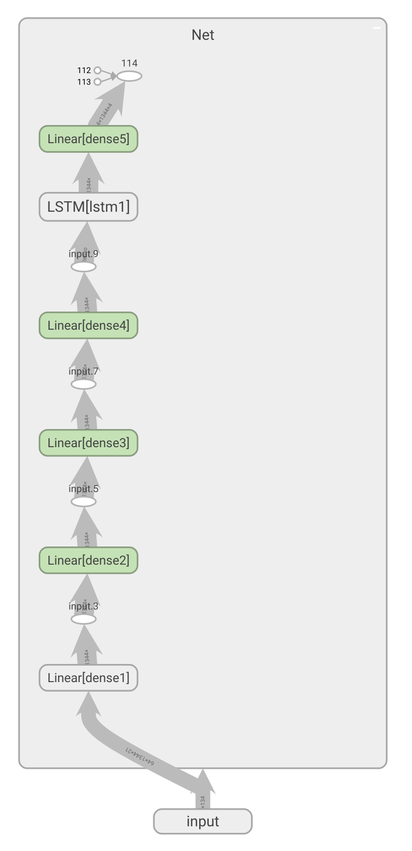
The network used in the project is relatively simple. Usually for speech recognition the network takes in multiple seconds of audio at a time. This allows convolution across time to extract features before feeding it into the recursive part. However, I decided that I wanted a streaming approach where the processing can happen in real time. Therefore I only used a few dense layers, followed by an LSTM to handle the temporal aspect of the decoding. This allows me to put in samples as they come in. The LSTM is followed by another dense layer and a softmax. The softmax outputs any of the letters in our alphabet or a special blank token.
Loss Function
The network will predict a probability for each token at each time step, see picture below. A simple way to extract the sequence from this is by taking the highest probability token at each time step, and then remove duplicate and blank tokens. An example sequence would look like “–H–E-LL–LLL–O–” (with “-“” for blank), which will turn into “HELLO”. There are better algorithms, such as beam search, but the greedy algorithm worked fine.
For training we don’t just need to extract a sequence, we need to compute a loss from the model output to the desired sequence. For this a Contortionist Temporal Classification (CTC) loss is used.
Real world results
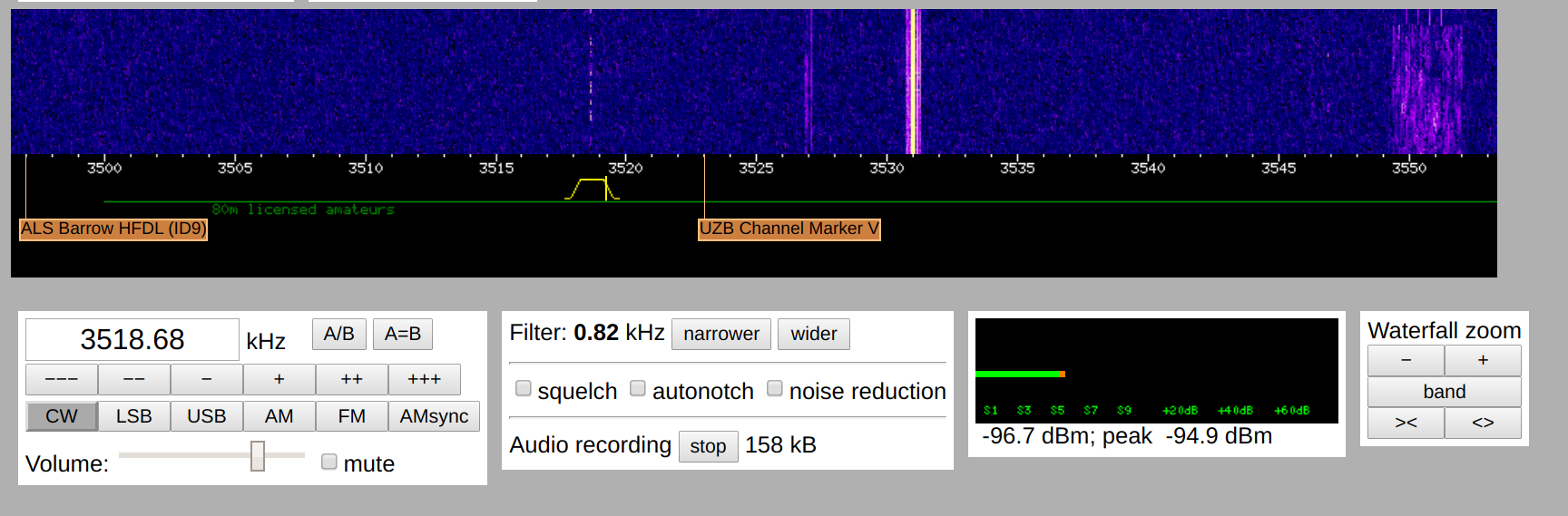
I let this model train for about half a day on a GTX 1070. At that point it had seen about 100 thousand examples segments of morse code. To test it’s performance on real world data, I used the on-line software defined radio from the University of Twente located in The Netherlands. I recorded some data on the 80 m band (3.5 to 4 Mhz), used by radio amateurs for morse code communications. Radio amateurs mostly exchange call signs on this band to prove they had contact. Let’s look at an example of a relatively weak signal.
The neural net decodes this as:
IV DE US5WAF HMTNXURRST559 55N OP YAR O Y ARO NR NR LVI E LVIV B W D+ DF3WV DE US5WAF I 4S5WAF DE DF3WV = TNX FR 55N UR RST 599 5NN ES NAME STEFAN STEFAN QTH RENNEROD RENNERON D = RIG F9 EEEEE F818 5WATTS 5 W = SOHW? BK BVDE USS MAF QTH ? QTH ? BK R BK QTS QTH RE N N E R OD
This is an interaction between US5WAF located in Ukraine and DF3WV located in Rennerod Germany.
The complete code can be found on my GitHub repo.